Stability

Equilibrium points

For autonomous systems with the property $f (0_{n×1})=0_{n\times1}$ the equilibrium points are the real roots of $f(x)=0$, which are points where starting at $x(0) = 0_{n×1}$ will remain there for all time.

If a system has an equilibrium point at an arbitrary point $\bar{x}$ we can simply define incremental coordinates $\tilde{x} = x - \bar{x}$, allowing the system to described by $f(\tilde{x}) = \dot{\tilde{x}}$, which has an equilibrium at $\tilde{x} = 0$.

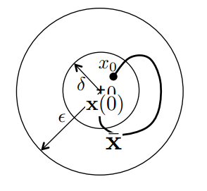
Stability

Origin is a stable equilibrium of $\dot{x} = f(x)$ if for each $\epsilon>0$, there exists a $\delta>0$ such that when $||{x(0)|| < \delta}$ $\rightarrow$ $||x(t)|| < \epsilon, \forall t \geq 0$

Summary: If initial conditions inside region $\delta$ the states will remain inside region $\epsilon$

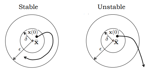
Asymptotic Stability

Origin is asymptotically stable equilibrium of $\dot{x} = f(x)$ if its stable and for $||{x(0)|| < \delta}$ $\rightarrow$ $\lim_{t\to\infty}$ $x(t) = 0$

Summary: If initial conditions inside region $\delta$ the states will converge to zero as time goes to infinity.

Asymptotic Stability

Lyapunov Stability

The origin is a stable equilibrium of $\dot{x} = f(x)$ if there exists $r>0$ and a positive definite function $V(x)$ on $B_r(0)$ such that $\dot{V}(x)$ is negative semi-definite on $B_r(0)$. Moreover, if $\dot{V}(x)$ is negative definite on $B_r(0)$ then the origin is asymptotically stable.

$\dot{V}(x)$ can be calculated using the chain rule:

Lyapunov stability can be summarized by the following conditions:

1. $V(x)$ is $C^1$, continuously differentiable
2. $V(0) = 0$ $V(x) > 0 \in \R \backslash0$
3. $\dot{V}(0) = 0$ $\dot{V}(x) \leq 0 \in \R \backslash0$

LaSalle's Invariance Principle

Positively Invariant Set

A set $\Omega$ is said to be positively invariant with respect to $\dot{x} = f(x)$ if $x(0) \in \Omega \rightarrow x(t) \in \Omega, \forall t \geq 0$

Summary: If you start in $\Omega$, you will stay in $\Omega$

LaSalle's Invariance Theorem can be used to show the asymptotic stability of an equilibrium when the derivative of the Lyapunov function $\dot{V}(x)$ is only negative semi-definite. \newline

• Let $\Omega$ be a positively invariant set with respect to $\dot{x} = f(x)$
• Let $V(x)$ be a continuously differentiable function on $\Omega$ such that $\dot{V} (x) \leq 0$ in $\Omega$
• Let E $\subset \Omega$ be the set of all points in $\Omega$ such that $\dot{V}(x) = 0$
• Let M be the largest positively invariant set in E

LaSalle’s Invariance Theorem

Exponential Stability

If there exists a function $V : D \rightarrow \R$ and constants $a,k_1,k_2,k_3 > 0$ such that

1. $V$ is $C^1$, continuously differentiable
2. $k_1||x||^a\leq V(x) \leq k_2||x||^a$
3. $\dot{V}(x) \leq -k_3||x||^a$

then $x = 0$ is exponentially stable.